Layered Cake Plot

A team is performing a cohort study to investigate health outcomes. The study will span a year, with patients being monitored monthly for any changes in their health.

To begin the study, the team will follow patients in the first month, collecting data on their health and well-being. In the following months, they will gradually add new patients to the study and continue to track the patients from previous months. This will help the team identify any changes in the health outcomes of patients over time and determine if there are any trends or patterns that emerge.

To display the patient count over time, the team could use an R-generated “layer cake” plot by using “tidyverse” package. This visualization method will enable the team to see how many patients are being added to the study over time and to identify any changes in patient numbers or trends. By using this visualization method, the team will be able to gain valuable insights into the data and make informed decisions about the study design and future research directions.

Suppose the structure of the data set is as follows:

So, we could create a layer cake plot by using tidyverse package as follow:

Code

# install.packages("tidyverse")
# install.packages("ggplot2")
# install.packages("viridis")

library("tidyverse")
library("ggplot2")
library("viridis") 

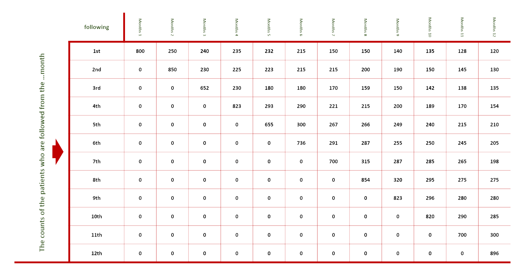
cohort.data <- data.frame(cohort=c('Cohort01', 'Cohort02', 'Cohort03', 'Cohort04', 'Cohort05', 'Cohort06', 'Cohort07', 'Cohort08', 'Cohort09', 'Cohort10', 'Cohort11', 'Cohort12'),
                          M1=c(800,0,0,0,0,0,0,0,0,0,0,0),
                          M2=c(250,850,0,0,0,0,0,0,0,0,0,0),
                          M3=c(240,230,652,0,0,0,0,0,0,0,0,0),
                          M4=c(235,225,230,823,0,0,0,0,0,0,0,0),
                          M5=c(232,223,180,293,655,0,0,0,0,0,0,0),
                          M6=c(215,215,180,290,300,736,0,0,0,0,0,0),
                          M7=c(150,215,170,221,267,291,700,0,0,0,0,0),
                          M8=c(150,200,159,215,266,287,315,854,0,0,0,0),
                          M9=c(140,190,150,200,249,255,287,320,823,0,0,0),
                          M10=c(135,150,142,189,240,250,285,295,296,820,0,0),
                          M11=c(128,145,138,170,215,245,265,275,280,290,700,0),
                          M12=c(120,130,135,154,210,205,198,275,280,285,300,896))

data <- cohort.data %>% pivot_longer( cols = -c(cohort), names_to = "month", values_to = "following") %>% mutate(month = factor(month, levels = c("M1",
                                                                                                                                                  "M2",
                                                                                                                                                  "M3",
                                                                                                                                                  "M4",
                                                                                                                                                  "M5",
                                                                                                                                                  "M6",
                                                                                                                                                  "M7",
                                                                                                                                                  "M8",
                                                                                                                                                  "M9",
                                                                                                                                                  "M10",
                                                                                                                                                  "M11",
                                                                                                                                                  "M12")))

#plot data
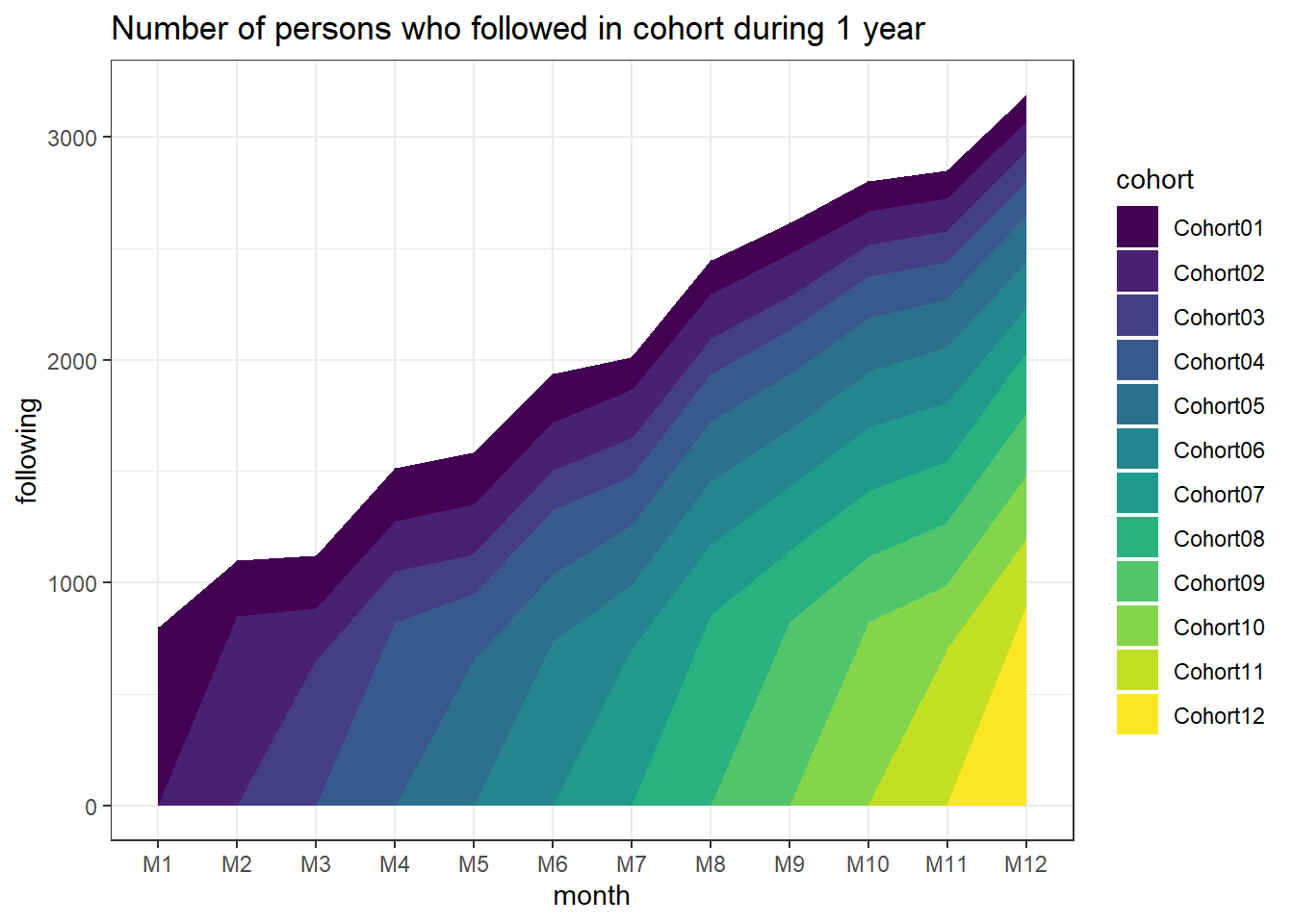
p <- ggplot(data, aes(x=month, y=following, group=cohort))
p + geom_area(aes(fill = cohort)) +
ggtitle('Number of persons who followed in cohort during 1 year') +
  scale_color_viridis(option = "D") +
  scale_fill_viridis(discrete = TRUE) +
  theme_bw()